
This model is a prototype version of a physical model for simulation of vehicle motion performance assuming a CVT gasoline vehicle.
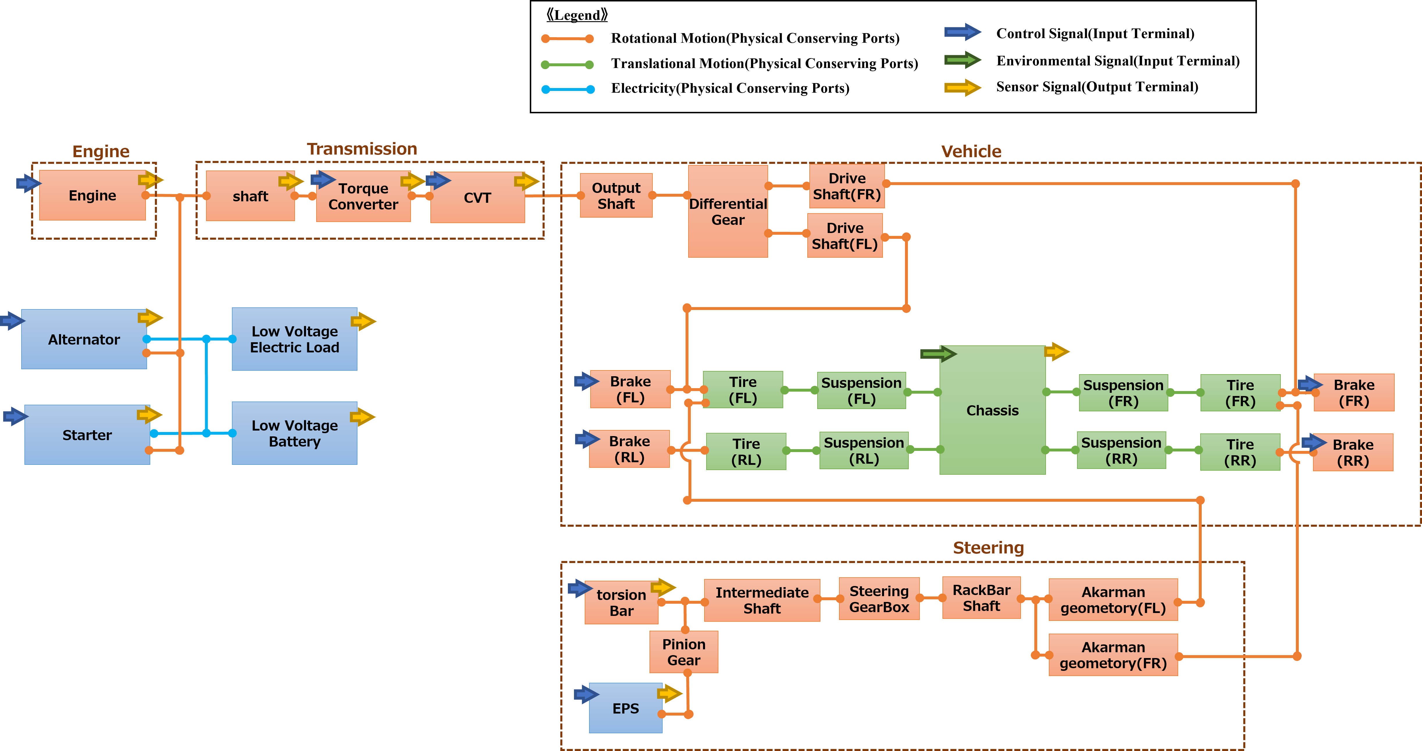
The powertrain consists of an engine (displacement 1.5 [L]) and a CVT.
The chassis consists of a steering wheel and a vehicle (4-wheel model with 3 axes / 6 degrees of freedom).
The electrical system consists of an alternator, a starter, a low-voltage battery, and an electrical load.
The chassis consists of a steering wheel and a vehicle (4-wheel model with 3 axes / 6 degrees of freedom).
The electrical system consists of an alternator, a starter, a low-voltage battery, and an electrical load.
Since it is a prototype version, everything inside the physical model cannot be edited.
* The product version is scheduled to be released on on this website website in November 2022.
Input / output signals are connected as follows.
Control signals and environmental signals are connected to the input ports.
Sensor signals and monitor signals are connected to the output ports.
There is no external connection to the physical conserving port.
Control signals and environmental signals are connected to the input ports.
Sensor signals and monitor signals are connected to the output ports.
There is no external connection to the physical conserving port.
List of signals:
・Control signals
Throttle opening, Idling stop flag,
Fuel cut flag, Ignition timing from MBT,
CVT pulley ratio, Torque converter lockup instruction flag,
Brake opening (4 wheels), Target motor torque,
Driver's steering operation torque,
Starter operation flag, Alternator target voltage
・Environmental signals
Road slope, Wind speed
・Sensor signals
Engine speed, Transmission output speed,
Low voltage battery SOC, Torsion bar torque,
Steering angular velocity, EPS motor angular velocity,
Vehicle speed, Yaw rate
* This physical model can be connected to the control model, which is a case study model in “Plant Modeling I/F Guidelines for Vehicle Development” published by the of Japan Automotive Model-Based Engineering center.
How to connect:
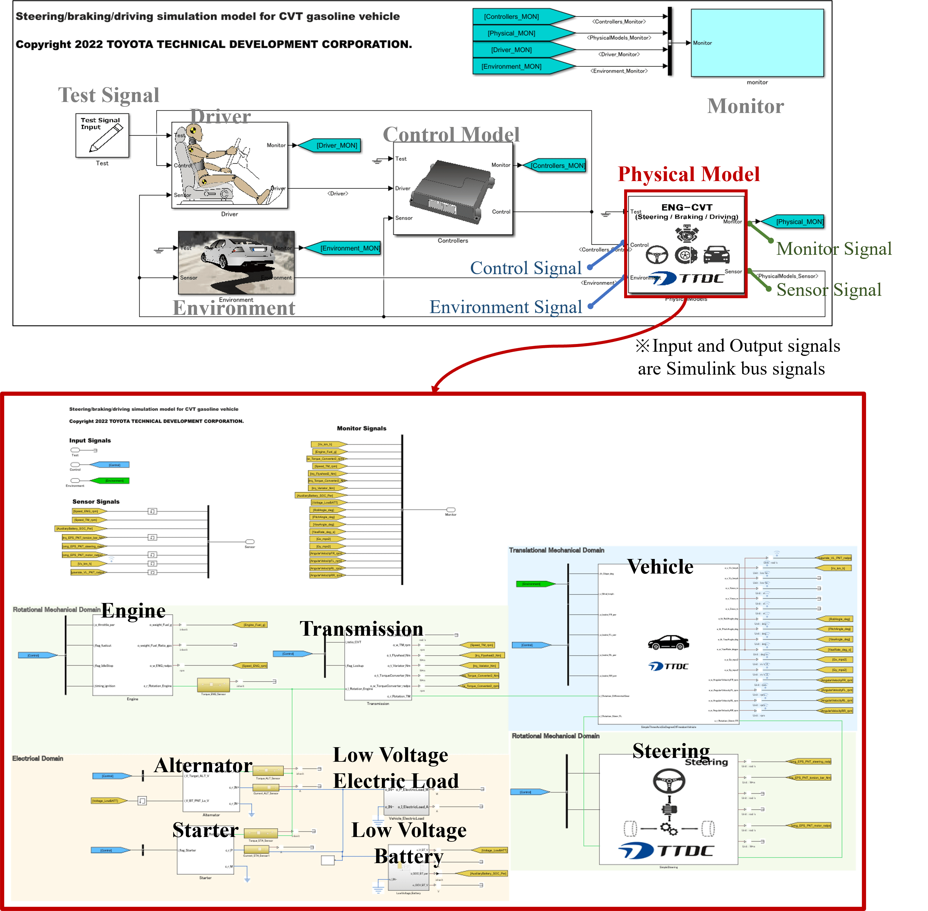
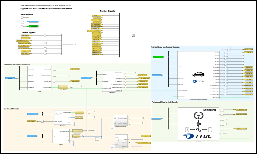
Internal configuration diagram:
The internal structure of this model is shown in the figure below.
Operating environment:

Block diagram :
Solver settings:
・ Global solver
- Solver: Arbitrary
- Sample time: Dependents on the setting value of the local solver
・ Local solver
- Solver: Backward Euler method
- Sample time: 2.5 msec
- Number of iterations: 3 times
- Solver: Arbitrary
- Sample time: Dependents on the setting value of the local solver
・ Local solver
- Solver: Backward Euler method
- Sample time: 2.5 msec
- Number of iterations: 3 times
Model constraints:
- This model does not simulate or guarantee the behavior and behavior accuracy of the actual machine.
- If the file structure in the library folder is changed, this model does not work.
- It may not work with other operating environments or solver settings than those listed above.
- It may not work with parameter sets other than those provided.
- The initial state is a stopped state.
- If the file structure in the library folder is changed, this model does not work.
- It may not work with other operating environments or solver settings than those listed above.
- It may not work with parameter sets other than those provided.
- The initial state is a stopped state.
How to execute:
1. Move the MATLAB current directory to the folder where the model files are located.
2. Execute the parameter file.
3. Open the model file.
4. Run the model.
2. Execute the parameter file.
3. Open the model file.
4. Run the model.