Download
Ver. 1.0.0
for R2021a

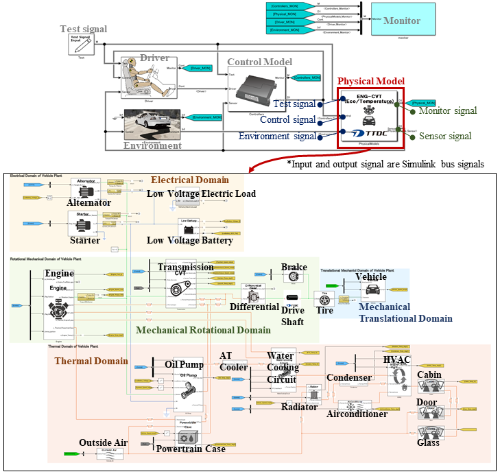
This model is a physical model of CVT gasoline vehicle. It simulates transmission control and thermal performance.
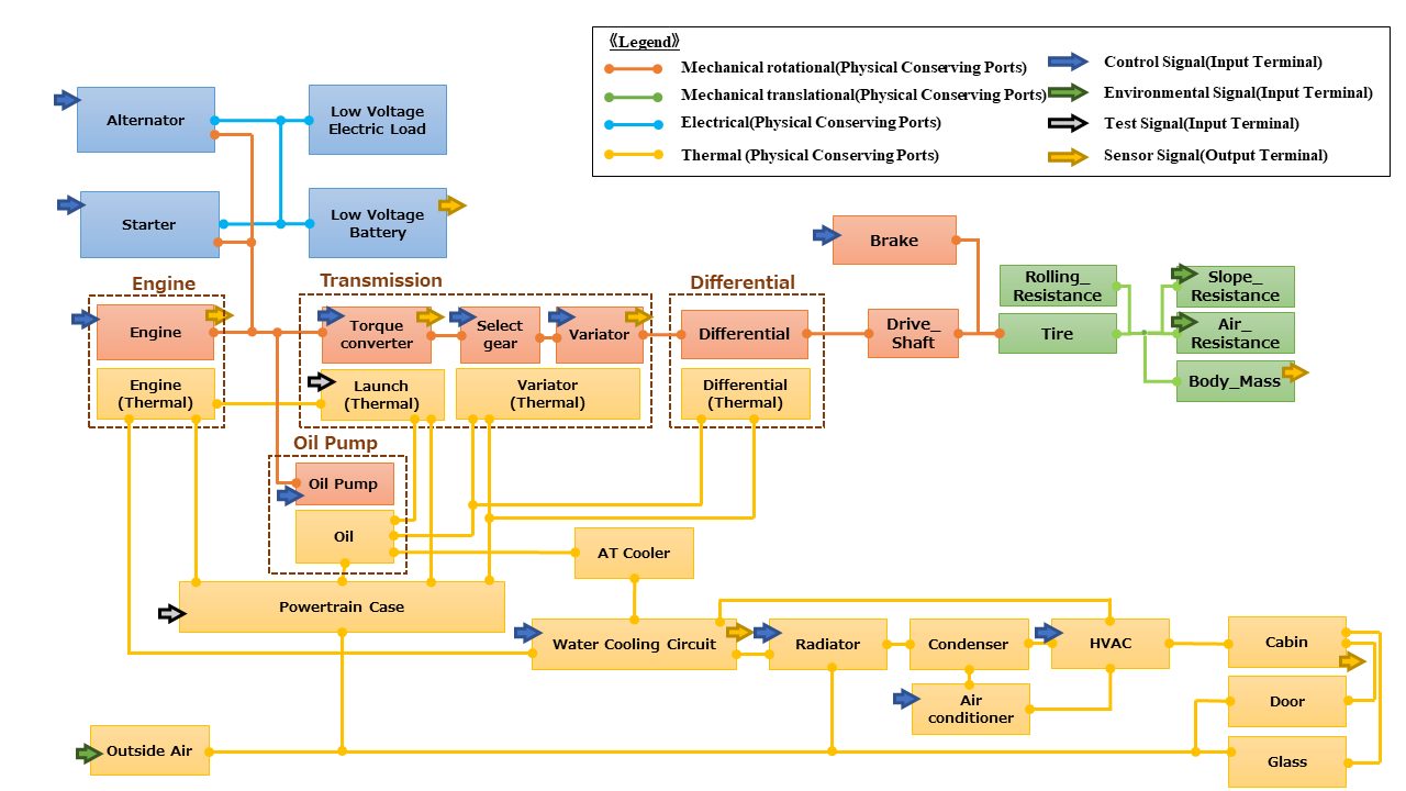
The powertrain consists of an engine (displacement 1.5 [L]), starter, alternator, transmission (CVT), differential, brakes, vehicle, and low-voltage battery.
The thermal system consists of a powertrain, oil, case, radiator, HVAC system, air conditioner, cabin, doors, glass, and water cooling circuit.
Input / output signals are connected as follows.
Control signals, environmental signals and test input signals are connected to the input ports.
Sensor signals and monitor signals are connected to the output ports.
There is no external connection to the physical conserving port.
Control signals, environmental signals and test input signals are connected to the input ports.
Sensor signals and monitor signals are connected to the output ports.
There is no external connection to the physical conserving port.
List of signals:
・Control signals
Throttle opening, Brake opening, Fuel cut flag,
Idling stop flag, Ignition timing from MBT, Hydraulic line pressure,
Clutch friction torque, CVT pulley ratio, Actuator current consumption,
Current consumption of electric oil pump, Valve opening of water cooling circuit,
Wind speed by radiator fan, Volumetric flow of water pump,
Heat flow of PTC heater, Heat flow of air conditioner,
Alternator target voltage, Starter activation flag,
HVAC fan voltage, Air mix motor voltage
・Sensor signals
Rotational speed of engine, SOC of low voltage battery,
Vehicle speed, Angular velocity of flywheel,
Angular velocity of gearbox input, Angular velocity of gearbox output,
Cabin temperature, PTC heater temperature, Cooling water temperature
* This physical model can be connected to the control model, which is a case study model in “Plant Modeling I/F Guidelines for Vehicle Development” published by the of Japan Automotive Model-Based Engineering center.
How to connect:
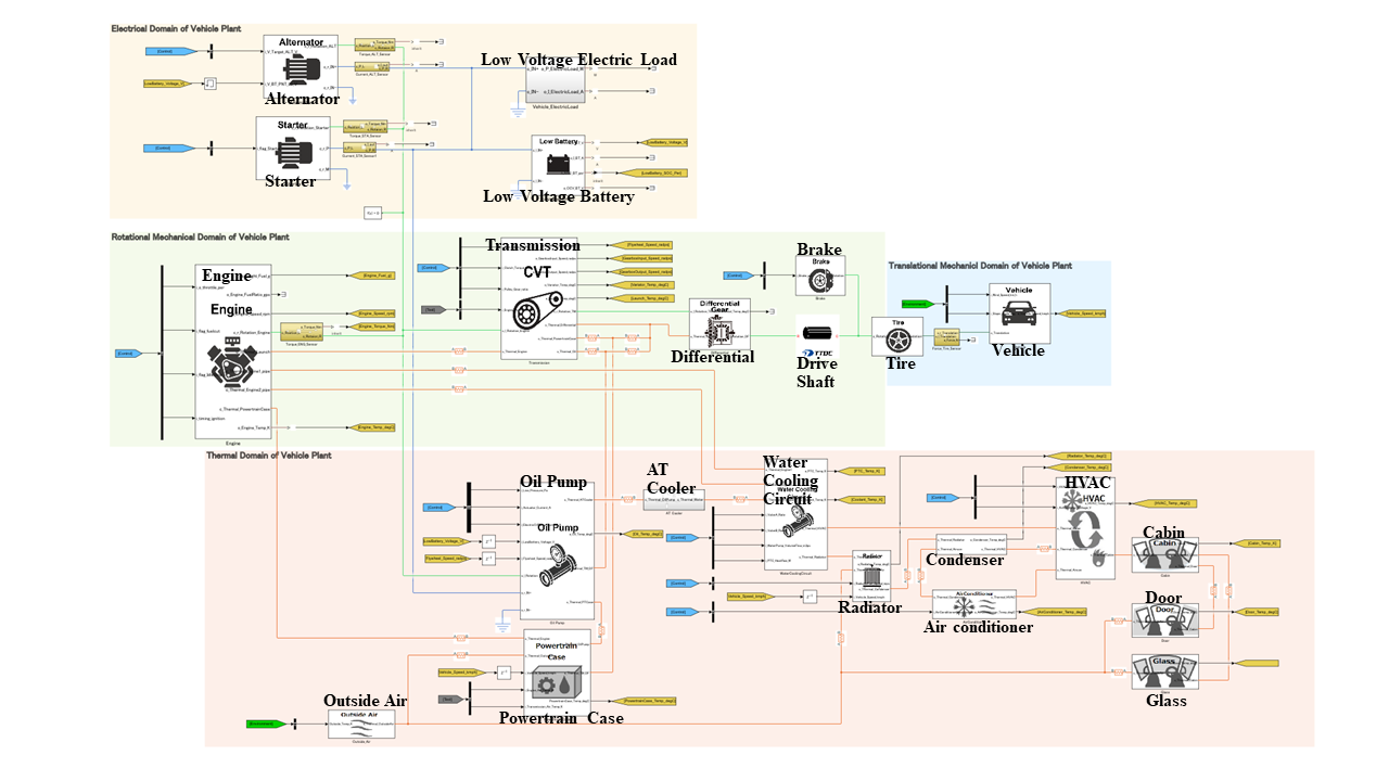
Internal configuration diagram:
The internal structure of this model is shown in the figure below.
Operating environment:

Block diagram:
Solver settings:
・ Global solver
- Solver: Arbitrary
- Sample time: Dependents on the setting value of the local solver
・ Local solver
- Solver: Backward Euler method
- Sample time: 2.5 millisecond
- Number of iterations: 3 times
- Solver: Arbitrary
- Sample time: Dependents on the setting value of the local solver
・ Local solver
- Solver: Backward Euler method
- Sample time: 2.5 millisecond
- Number of iterations: 3 times
Model constraints:
- This model does not simulate or guarantee the behavior and behavior accuracy of the actual machine.
- If the file structure in the library folder is changed, this model does not work.
- It may not work with other operating environments or solver settings than those listed above.
- It may not work with parameter sets other than those provided.
- The initial state is a stopped state.
- If the file structure in the library folder is changed, this model does not work.
- It may not work with other operating environments or solver settings than those listed above.
- It may not work with parameter sets other than those provided.
- The initial state is a stopped state.
How to execute:
1. Move the MATLAB current directory to the folder where the model files are located.
2. Execute the parameter file.
3. Open the model file.
4. Run the model.
2. Execute the parameter file.
3. Open the model file.
4. Run the model.
Download
Ver. 1.0.0
for R2021a
Ver. 1.0.0
for R2021a